Induction Circuits

by Kyle Smith on 2025-03-01

Induction, the process of bringing about or giving rise to something, is one of the key internal mechanisms discovered in large language models (LLMs). Put simply, LLMs can detect and extend repeating patterns in text (during inference). This ability is part of what is more commonly seen as in-context learning. For example, when given the prompt: The vision of Apple was conceived by Steve Jobs. Steve ..., the model looks back, notices that Steve was followed by Jobs, and predicts Jobs again. While this may seem obvious, it reveals a deeper question: how do models actually implement such behavior internally? We know that LLMs solve the task of predicting the next token based on prior context, but beyond simple n-gram models, they learn far more complex, long-range relationships using attention and backpropagation. What algorithms emerge inside the model to support this? In this blog, we'll explore one such algorithm: induction circuits. To do so, we'll dissect a small GPT-2 model using the excellent TransformerLens library—my wallet is GPU-poor, but curiosity is free.

What we will discover:

1. The exact mechanisms of induction circuits inside a GPT-2 model.
2. How information is packaged and transported between the layers of the model.
3. The suprising effectiveness of the residual stream and how it encodes information.

To understand induction circuits, we first need to take a deeper look at the transformer found at the heart of the GPT-2 model:

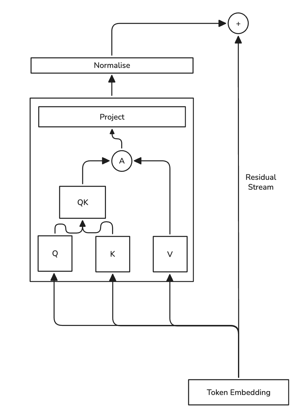Figure 1: GPT-2 Transformer

Let A represent the operation of calculating the attention scores and normalising them ().

The key component that differentiates transformer models from typical deep neural networks are the attention blocks. In a decoder-only model like GPT-2 they empower the model to learn uni-directional relationships between tokens, allowing the model to relate a token to another token earlier in the sequence. This is what allows models to learn how to perform induction during the prediction process. However, the real magic lies in the residual stream, we will see the residual stream plays crucial role in the propogation of information through the layers of the model. The residual stream is more commonly referred to as a skip-connection when talking about classic deep-learning models such as deep neural nets or CNNs. It was simply a technique to facilitate stable gradients through the network during optimisation. However in the context of transformers, it plays a much more abstract role, as argued in the paper A Mathematical Framework for Transformer Circuits, the residual stream is actually the main mechanism in which signals are carried through the model, rather than the transformer blocks themselves. For a real-world analogy the residual stream can be thought of as the conveyor belt in the assembly line and the attention heads as the stations where specific parts are added to whatever is fed into it. The residual stream can be thought of as the enrichment of the original token embedding, where after enrichment the token is finally morphed into the predicted token.

Now instead of taking this argument as face value, let's try and see if we can see this behaviour in the model. Specifically let's look at the residual stream values after applying feeding it through the transformer block.

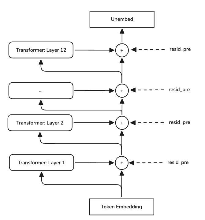Figure 2: Residual stream activation points

To easily capture the activation values at these points we will use the TransformerLens library.

def get_project(attention_out):
  # pass attention through final linear layer to
  output = gpt2_small.ln_final.forward(attention_out)

  # unembed the representation from the linear layer to an embedding representing a token
  unembed = gpt2_small.unembed.forward(attention_out)

  # apply softmax to 'score' each predicted token in the range (0, 1)
  norm = t.softmax(unembed, dim=-1)

  # choose the one with the highest score
  top = t.argmax(norm, dim=-1, keepdim=True)

  # conver the embedding to a string using gpt2 tokenizer
  return gpt2_small.to_string(top)

input = "Steve Smith is the chief visionary behind Gig. Steve Smith is"
gpt2_small: HookedTransformer = HookedTransformer.from_pretrained("gpt2-small")
input_tokens = gpt2_small.to_tokens(input)
logits, cache = gpt2_small.run_with_cache(input_tokens, remove_batch_dim=True)

for i in range(12):
  activation = get_project(cache["resid_post", i])[1:] 

The get_project function takes as input the residual stream activation and will then attempt to decode the activation into a string token by feeding the activation directly into the output layer of the model. This is not neccessarily correct and was done as a experiment, but turned out to be a nice approximation of which token the activation currently encodes. The input sequence is strange, but that is intentional, it is just my attempt to confuse the model. I purposefully wanted to use an example where the firstname could refer to a well-known figure such as Steve Jobs or Steve Martin, to see if the induction circuit would overwrite these values when Steve appears later in the input. Below you can see how the tokens were transformed in the model during inference:

What we are seeing above is how the tokens are transformed through the various transformer blocks. The final token in the list is what the model predicts should follow the highligted token. This gives a small (and not perfect) glimpse into the reasoning process of the model, but we are here for induction circuits. So for the first token (Steve) the model with its limited context thinks we are talking about Steve Jobs, so it predicts that Jobs should follow Steve. So at this point no induction is performed since it does not really have context. However, if you select 9 in the dropdown you'll see it actually predicts that Smith should follow Steve. Now that we can see that induction action, we can delve deeper into how the model is actually doing this.

For simplicity we will be investigating induction circuits which perform exact matching as opposed to fuzzy matching. For an exact matching induction circuit it needs to be able to do two things:

1. It needs to know if there is a repeated sequence of tokens in the input (prefix matching).
2. If there is a repeated sequence of tokens then it should copy the token that follows the repeated token (copying). We will find this behaviour embedded in the attention heads.

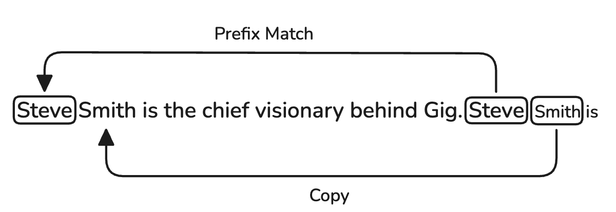Figure 3: Induction on sequence

Assume the model is trying to predict Smith, the induction circuit will then perform two actions:

1. First it will recognise that Steve is typically followed by Smith and so it will assign a high attention score to Steve.
2. This attention score then signals to an attention head in a later layer that it should 'boost' the attention score of Smith, effectively copying it. The above two actions can be idenified in two heads, as the behaviour can typically be found in an attention head.

So to see this in action, let's write two function to help us identify specific attention patterns in the model.

def prefix_matching_head_detector(cache: ActivationCache, original_token_idx, prev_token_idx) -> list[str]:
    detected = []
    for i in range(model.cfg.n_layers):
      pattern = cache["pattern", i]
      for (idx, head) in enumerate(pattern):
        if head[original_token_idx, prev_token_idx] > 0.6:
          detected.append(f"{i}.{idx} - {head[original_token_idx, prev_token_idx]}")

    return detected

The above function will find all heads where the head assigned a value greater than the configured threshold value between the pair of tokens at the indices original_token_idx and prev_token_idx. It will output a list of the form where the value before the '.' is the layer index and value after is the head index. The value after the dash is the attention value. Running the code above on the activation values from our chosen sequence to find the prefix matching heads, i.e. the heads that assigned a high attention score to the first occurrence of Smith when trying to predict what comes after the second occurrence of Steve, we get:

['5.5 0.8519402146339417',
 '6.9 0.8816268444061279',
 '7.10 0.7206246852874756',
 '10.0 0.5999936461448669',
 '10.1 0.41238731145858765',
 '10.10 0.42451727390289307',
 '11.10 0.42704296112060547']

This is interesting, because if we look back at the token layer transformations, when Steve is highligted the token is transformed to Smith somewhere around layer 7 (index 6) or 8 (index 7). Which actually aligns with what we are seeing in the attention scores for that token. The attention scores seem to indicate that the Smith token is carried between layers 6-8 and then appear later in the final two layers. Now we can't yet reason as to why exactly this is happening, but we can try. Before we do that, we need to gain a better understanding of how the residual stream organises information.

The residual stream dicates the result of the predicted token, more specifically the state of the stream dictates the current token that will be predicted. The state of the stream can be described as the contents of the 768-dimensional vector, which is the width of the vector in the case of the GPT-2 model.

More formally a single representation for a token can be decomposed into a set of subspaces, where each subspace encodes some specific piece of information. More specifically a subspace would be a set of vectors representing some useful concept (in the case of LLMs). Intuitively if you consider the physics definition of a vector: "Representing a force that has magnitude and direction. Each direction represents a concept or piece of information and the magnitude in that direction represents another piece of useful information in the context of that direction. For example one vector (one arrow) would represent the token embedding and another would encode the positional information. These vectors would then live in the token embedding subspace and positional embedding subspace which in turn form part of the residual stream embedding. To make this more concrete consider what we did to get the tokens in token layer transformations. We took the embedding for each token in the sequence and unembedded it to get the token representation. This process was performed by projecting the latent embedding with the unembedding matrix, we are thus extracting only the token information from the embedding. Think of it as extracting from the model's internal language the bits of information we care about(not exactly, but you get the point). So to visualise subspaces we consider our initial emebedding vector, which holds the position embedding and token embedding:

So in the simplified example above, we have a 2D vector (think (x,y)), where one component represents the token subspace and the other component represents the position subspace. This idea generalises as we increase the dimensionality of the vector. Furthermore, you'll notice that the subspaces are orthogonal, this is usually what is desired as they allow for cleaner projections, but are not strictly required (and is unfortunately rarely true). This is actually one of the key challenges in interpreting LLM models, as the model learns more complex projections which mix subspaces making them difficult to interpret (this problem is due to superposition see 1). The mixing means, the subspaces are not exactly orthogonal. But with that we can actually start to construct the blueprint for the induction circuit.

Let's look at our example sequence:

Steve Smith is the chief visionary behind Gig. Steve Smith is

This sequence is first tokenised to get the token IDs, which means it is translated to a list of numbers that looks something like this:

12 32 ... 12 32 102

Each token is then passed to the first layer in the model (the embedding layer), a lookup table which is then used to find the corresponding embedding for a token. Then for simplicity we assume the positional embedding is added, which is responsible for recording the position of the token in the sequence. Effectively creating a second subspace in the embedding vector, which means we get something like the following:

Now these embeddings are given to a transformer to produce a new transformation of the current latent embedding which added back to the residual stream (recall Figure 2). Now we need to take a look at the transformer block again, specifically the attention mechanism (just because that is where the most interesting stuff happens):

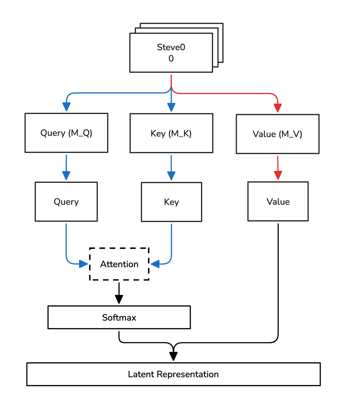Figure 6: Attention Mechanism

So when processing the embeddings of a sequence, each token is projected into three different spaces:

1. The query space with the matrix , where the resulting matrix after projection is denoted as .
2. The key space with the matrix , where the resulting matrix after projection is denoted as .
3. The value space with the matrix , where the resulting matrix after projection is denoted as .

Each matrix holds a representation for each token in the sequence. So the dimensionality of each matrix will usually have dimensionality where is the length of the sequence and is the head size (usually equal to the dimension as the residual stream). The equation for a simple attention mechanism can be given as:

The numerator represents the attention score calculation, an attention score is a numeric value indicating how relevant a previous token is to the current token.
To understand what this means, let's look at a simplified version to understand what the matrix multiplication is actually doing:

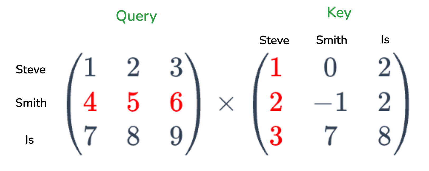Figure 7: Query Key Calculation (Snippet)

In Figure 7 we have a Query and Key matrix for the first three words in our example sequence. has an embedding length of 3 and an important caviat is that in auto-regressive LLM models such as the GPT-series models, we can only attend to tokens that appear before the current token. So Smith can only attend to Steve in this toy-example. What we are checking is if the query embedding for Smith is relevant to the key embedding Steve (imagine how a DB query might use a key in an index). This gives as a single attention score, this is repeated for every token in the sequence. This gives us an attention matrix, where a single element tells us how relevant a token is to another token. The $softmax$ operation is applied so that the attention scores are clamped to be between 0 and 1, where a value closer to 1 indicates higher relevance.

So let's stop for a moment and think what the attention calculation is really trying to achieve. This calculation captures the relationships between tokens, the type of relationships might be syntactical such as relating a determiner with a noun, or more abstract relations such as "dog" relating to "animal". Each layer might be responsible capture a different set of relationships. For the induction circuit we simply want to attend to the token before the current token. The type of relationship extracted is parameterised by the matrices and . So in the context of the induction circuit, one of the types of relationships that might cause a high attention score is assigning a high score to a token that is directly before the current token. For example, a hypothetical attention score matrix might look like:

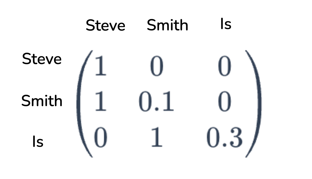
So in this case Smith has a relationship with Steve, so this will cause this piece of information to be encoded into a subspace when multiplied with the Value matrix.

The attention matrix is then multiplied with the Value matrix . Since the attention matrix values are between 0 and 1, we can think of the attention matrix is exciting or masking certain subspaces of the value matrix embeddings. This can be visualised as information being added and removed from subspaces in the Value matrix. So in a perfect world the embeddings after the first layer in an induction circuit will look like the following:

Also this is not necessarily the first layer in a model such as GPT-2, as we saw when we tried to find the induction heads, we saw that there were multiple places where this occurred. So now this information will be added into the residual stream (the output of the attention block is technically fed into another Linear layer, but the information will still propogate through). Another head might decide to overwrite this subspace, but some heads might completely ignore it (which is pretty cool). Now the earlier Smith token helped encode the fact that it is the successor of the token Steve. Now the next part of the puzzle is that it needs communicate to next Steve embedding that it was previously before Smith. This step is a bit abstract and was a bit difficult for me to see and visualise, but what happens is something like the following:

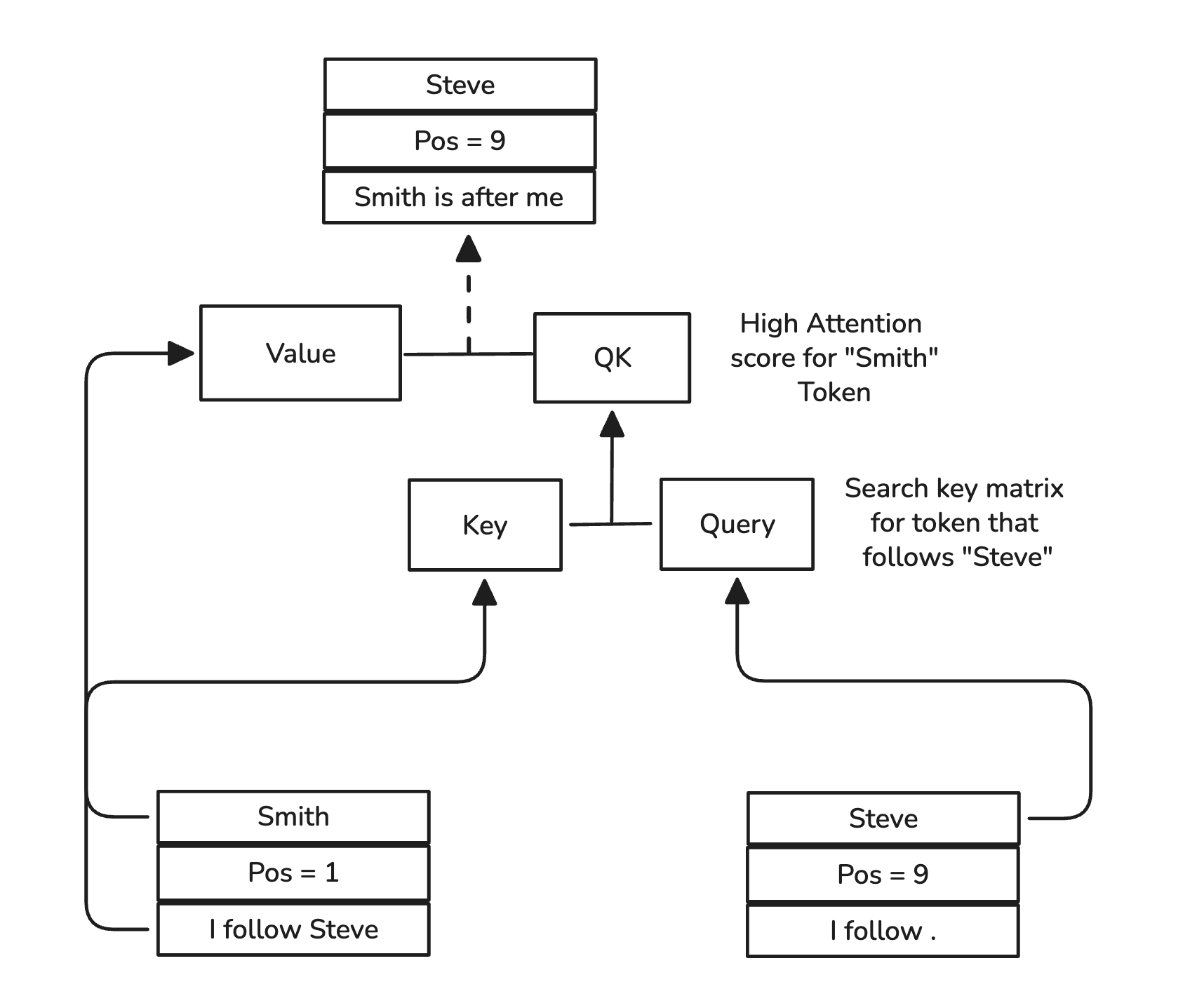Figure 8: Final Induction Circuit Step

So the strange part here is the final matrix multiplication and the value matrix (full calculation left out for simplicity) where the subspace I follow Steve is read and through the multiplication with the attention score matrix it transforms that subspace into a new xxx is after me subspace. So it is interesting how these two values encode a whole new piece of information.