What makes good image features?

by Kyle Smith on 2026-08-08

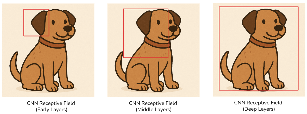
During the breakthrough of deep learning around 2012, the deep convolutional neural network AlexNet was considered the gold standard. The CNN architecture still remains a very solid architecture, as they are generally efficient, powerful and can be used for almost every computer vision task. CNNs are trained to develop their own feature extractors through parameterised kernels. As found in this article by Anthropic, CNNs in the earlier layers optimise kernels to identify basic geometric features such as lines, curves etc. These features form the basis of a hierarchy of features that become more and more abstract.

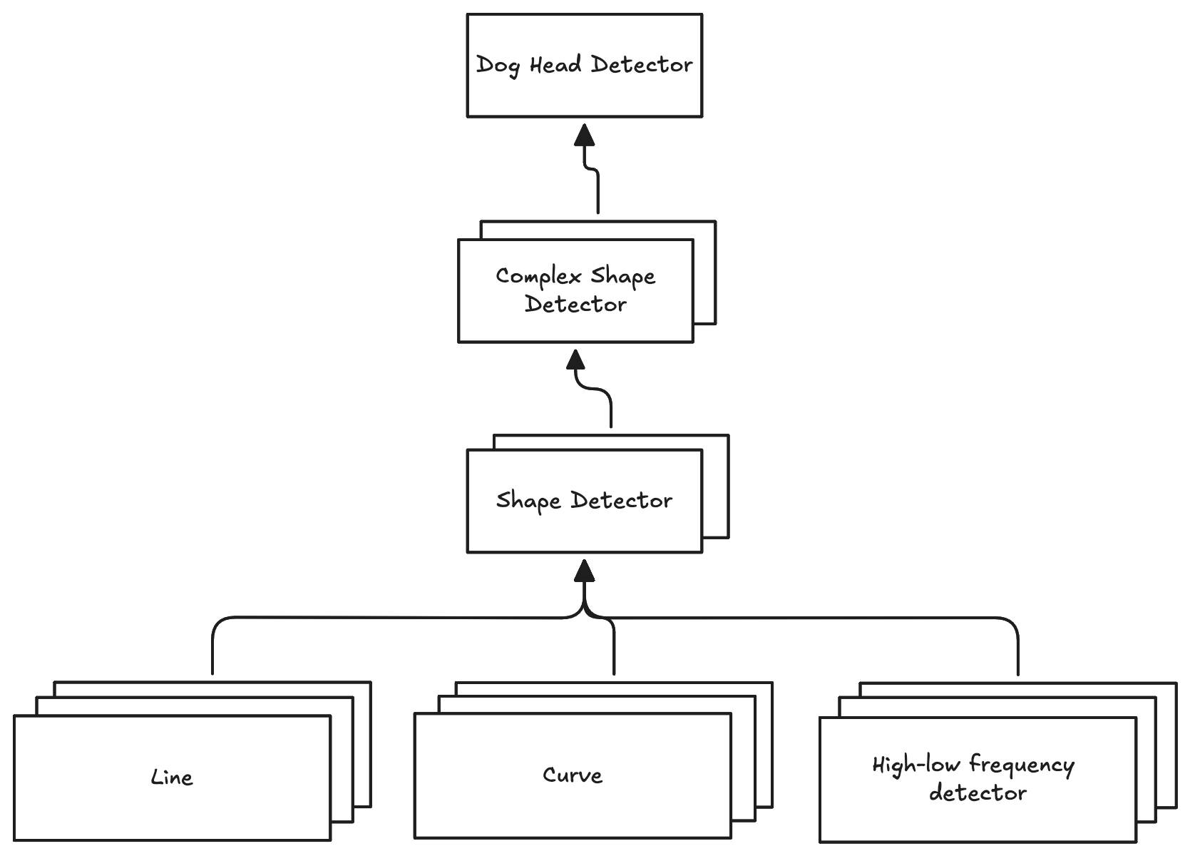Figure 1: A hierarchy of increasingly abstract CNN features

More recently LLMs have popularised the concept of foundational models that are powerful generalists that can either be fine-tuned or, with some smart prompting, be adapted to a specific use case. This raises an interesting question: could you build a foundation model that could be adapted to computer vision tasks? Well, as some smart people at Meta have shown, yes you can.

DINOv3 is a powerful image backbone that, with the addition of some neurons to decode the detected features, can be used for object classification, object detection, depth estimation, semantic segmentation, 3D scene understanding etc., achieving close to state of the art. Now the interesting question becomes: what features does the model output that are so useful?

For a model to be a good generalist, two things are required: a diverse and large training dataset and dense features. The first point makes sense, since the more data we have the closer we can approximate the theoretical data distribution (assuming the model has enough parameters). To understand the second requirement we first need to understand: what is a feature?

When describing a feature in a "literal" sense it can be described as a vector in some high dimensional space. In other words a feature is a line describing the magnitude and direction in some feature vector space. They occur as the activations in the individual layers of a model. Typically a positive activation (think ReLU activation function) means a feature that neuron is tasked with identifying exists, and negative if the opposite (this is not exact, but still useful for understanding). Take this simple neural network:

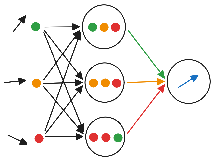Figure 2: Composing features in a simple network

In this model we describe a neuron (a circle) as identifying a single feature. A neuron is parameterised by the weights which connect to it (the arrows). We show activation strength as colour (green == max, orange == mid and red == low). A neuron before activation is a linear combination of input features (different combinations of colours in the circle). This is how features are composed. The linear combination is represented as a scalar value (with a dot product) which is then fed to an activation function to determine the activation strength. This can be combined with other neuron outputs to create a new abstract feature (blue arrow).

For a more mathematical view, we reframe features as vectors and weights as matrices.

The input for the first neuron is computed as $\begin{pmatrix}x_1,x_2,x_3\end{pmatrix} \cdot \begin{pmatrix}w_{11},w_{12},w_{13}\end{pmatrix}$, which tells us how aligned the vector containing $x$ is with the weights. The greater the alignment the higher the activation.

In actuality a vector in a neural network might represent multiple features due to the network needing to compress information (this property of neurons is called polysemanticity). A direction in the feature space typically aligns with some meaningful aspect relating to the dataset or task the model is being used for.

Features in image related tasks range from simple geometric shapes such as lines or curves to more abstract objects such as dog faces or car wheels. In the case of an object classification task, later layers might learn to excite when features are given that match some object from the dataset such as a dog, car etc. The magnitude of the feature vector can usually be related to how "confident" the model is in a particular feature.

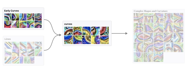Figure 3: Later layers respond to more abstract, object-level features

This notion of abstraction in earlier layers has been found to be more prominent in CNNs. In the ViT architecture you actually end up getting more semantic features in earlier layers, which lends itself to being more attractive for the case of a generalist vision backbone.

The vision transformer architecture takes inspiration from its NLP cousin the LLM by treating images as sequences of data. Instead of trying to establish feature extractors like a CNN would, it divides the given image into a sequence of patches (equal non-overlapping slices of the image). The idea is that the model can then learn relationships between these patches through the attention mechanism in the transformer block.

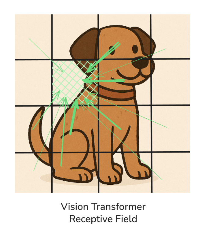Figure 4: An image split into a sequence of patches (source)

The architecture is described in the image below:

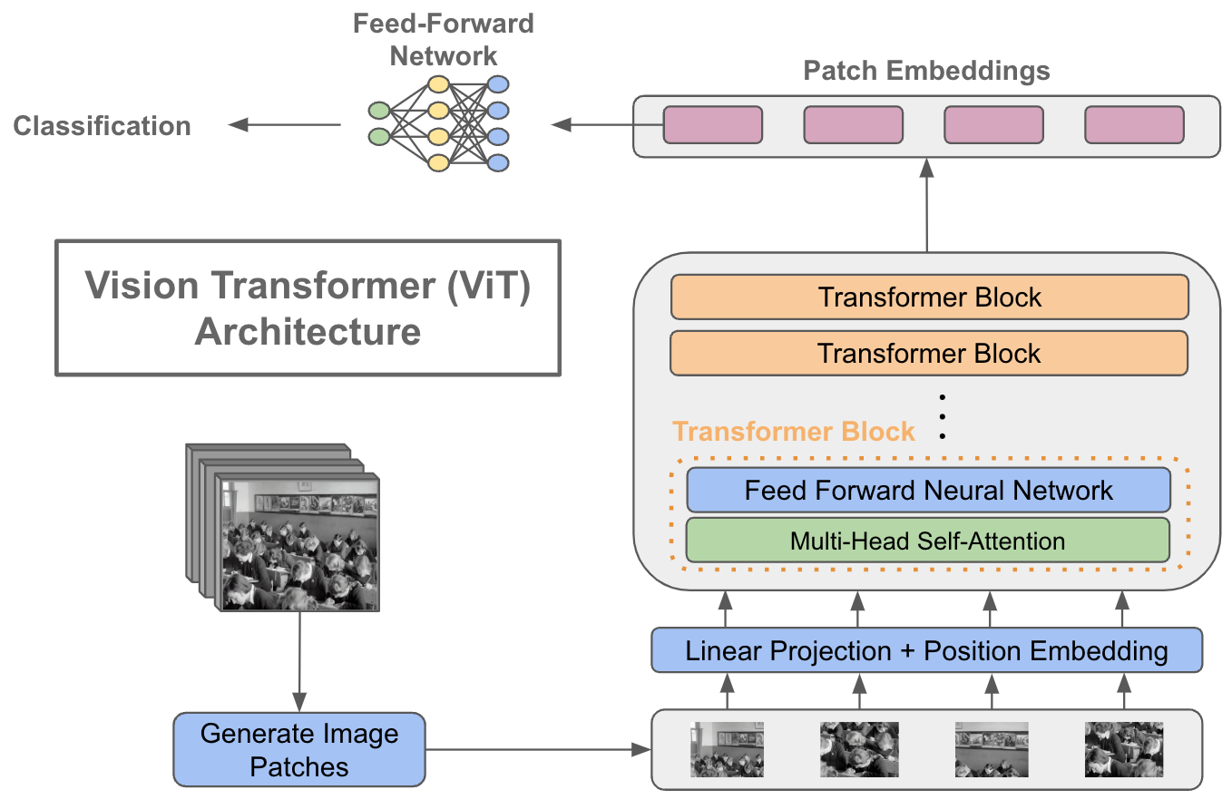Figure 5: Vision Transformer architecture (source)

The interesting point here is that ViT models learn the relationships between the patch embeddings. The idea is that the model can learn that certain patches represent ears, an animal body etc., and then later layers can stitch these features together to identify what type of animal is in the image.

We can visualise this by comparing the patch embeddings to see how patches are related to each other. Taking this example of a cat, you can hover over different parts of the image to see how closely related the patches are — notice how patches on the cat itself light up together. Here I run DINOv3 (ViT-S/16) over the image, take the final-layer patch embeddings, L2-normalise them, and compute the cosine similarity between the hovered patch and every other patch.

Visualising the patch embeddings is great and tells us an interesting story of how patches are related to each other to form semantic groups. Now let's take a look at the geometry of embeddings, to understand how the features are encoded.

The superpower of AI models is that they are experts in storing and compressing information. This information is usually visible in the dataset that the model was trained on and should represent, to a certain degree, the data the model will be tested on. AI models have the goal of trying to learn features such that they can cleanly separate data. Features are learned representations of data. One theory explored in Topology of Deep Neural Networks is that models attempt to learn transformations that can separate the data linearly. Take this toy dataset where you want to classify points on whether they sit on the inner or outer circle:

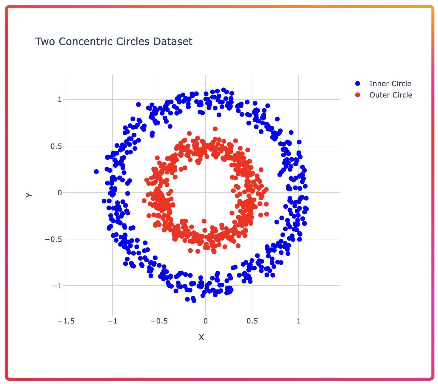Figure 7: A dataset that is not linearly separable

A trained neural network with enough layers will end up finding a way to transform the points into the following arrangement:

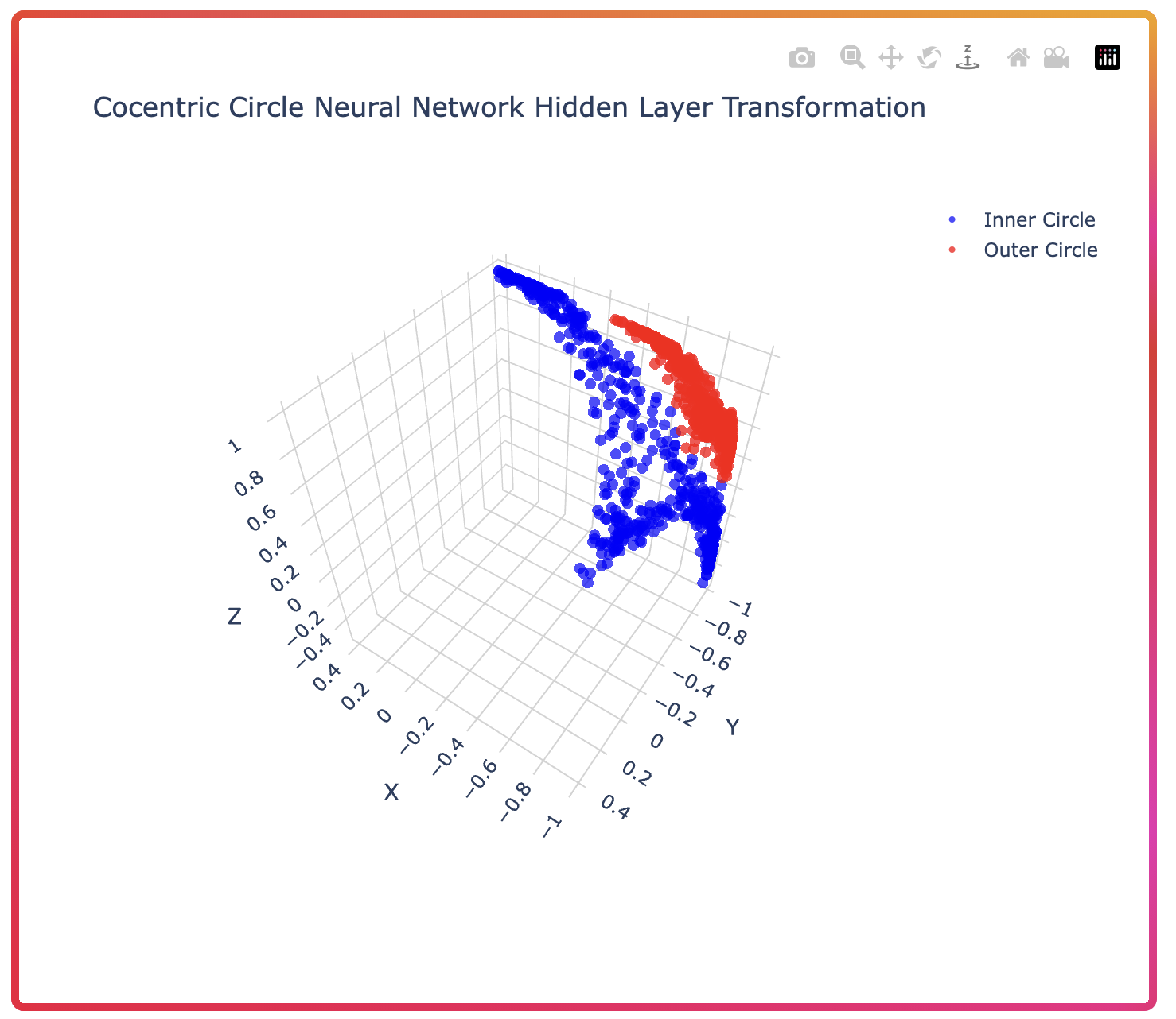Figure 8: The same points, now linearly separable

Notice how the class of the points has not changed, but you can see the points can now clearly be separated (imagine placing a piece of paper between the blue and red clusters).

Now to relate this idea to images, we first need to imagine how we would represent an image in a higher dimensional space. Assume we only consider 224 × 224 RGB images. The image will then have 50,176 pixel values. So an image can then be plotted as a point in 50,176-dimensional space. The way in which the model manipulates the points in the space depends on the data it is trained on and the task it is being trained for. The challenge is that, due to the high complexity of images and the large number of factors which can impact how an image can look, the points might be knotted in a complex way:

Figure 9: A simplified view of data manifolds for a binary classification task

The image above provides a simplified view of a neural network trained on a binary classification task. The blobs are called manifolds; a manifold represents a collection of data points. So you can imagine your dataset has a complex geometry that can be described by a set of manifolds that are connected in a meaningful way. The idea is that the data points in a dataset can be sampled from some manifold, and that data points which are related lie on the same manifold. I don't fully understand manifolds so won't describe exactly what they are, but the visual above should be enough.

Now you might be wondering how features play into this idea that data has a geometry. Consider we have some manifold $\mathcal{M}$ that represents all images of cars. A model might learn a set of vectors $f$ that actually parameterise the manifold. To visualise this, assume you look at a random image that lies on the manifold. You can then walk the manifold in any direction and see slight variations in the image (this is called the tangent space). The idea is that directions on this manifold correspond to features.

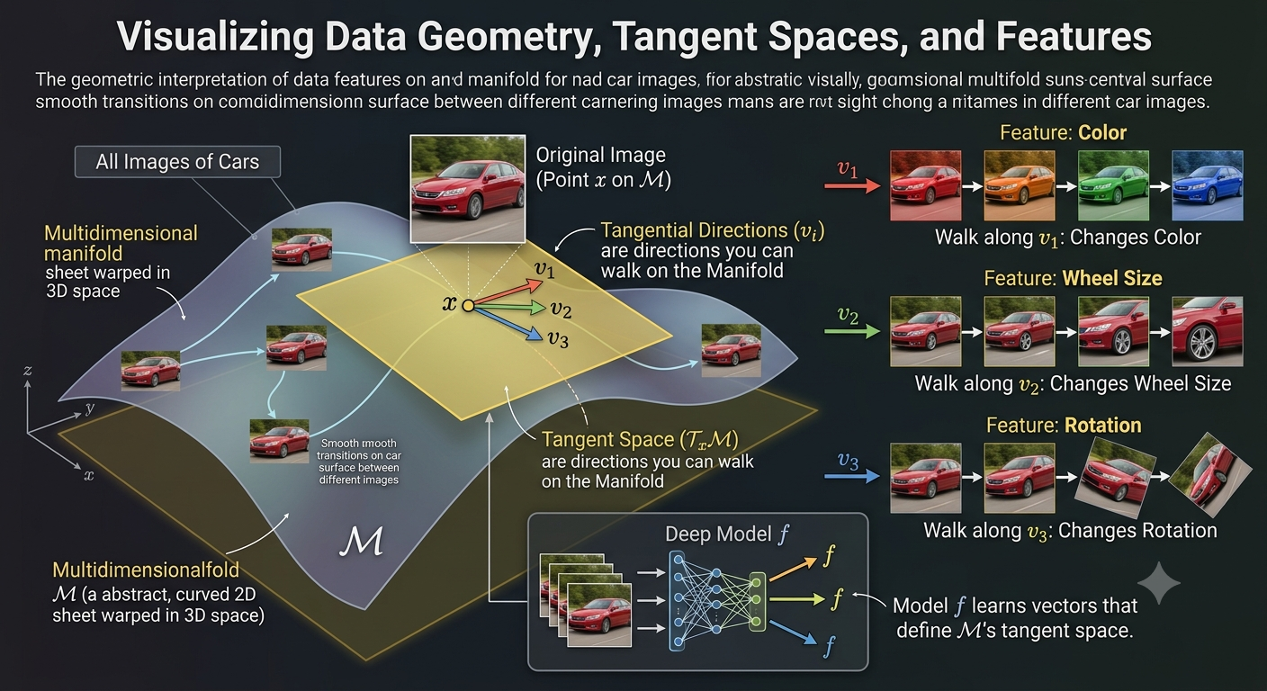Figure 10: Directions along a manifold correspond to features

In the context of the DINOv3 model, it learns a series of embeddings $z_i$ of patches of a given image. Each embedding can be decomposed into a direct sum of semantic subspaces, where a subspace is a collection of related features.

I believe the subspaces might be the key to understanding dense features. My hypothesis is that an embedding has an effective dimensionality that consists of a series of subspaces, each subspace encoding some collection of related features. As described in this paper by Anthropic, models prefer to represent correlated features as orthogonal and anti-correlated features as being in opposite directions.

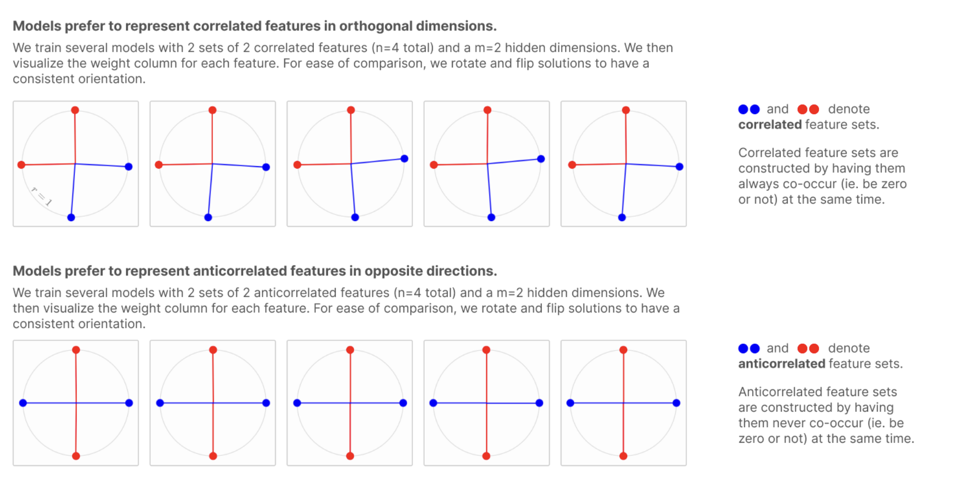Figure 11: Correlated features arranged orthogonally

However, due to models being forced to compress data, they can't always organise features to be orthogonal. So if correlated features can't be organised as orthogonal, then they are placed side-by-side.

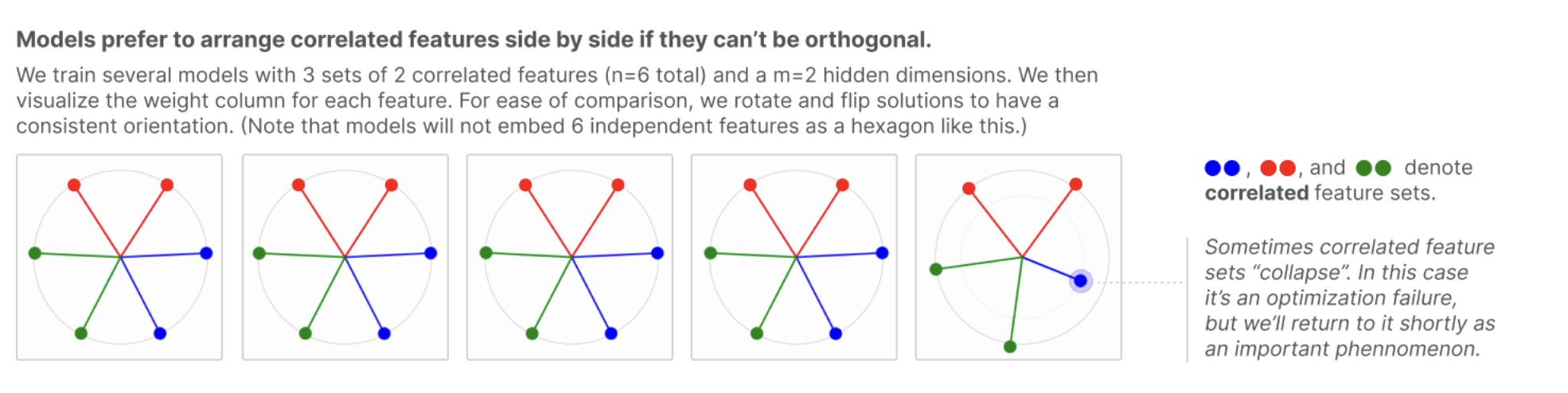Figure 12: When orthogonality isn't possible, features are packed side-by-side

So this answers the question of how DINOv3 could potentially organise the features within subspaces.

For DINOv3 to be effective at different downstream tasks it needs to have a very rich embedding. As we saw with the patch embeddings visualisation, the embeddings of semantic objects were similar. This shows that the model is able to capture the semantic objects and pack them into the embedding.

Using a quick experiment we use the scene-150 dataset from HuggingFace. This helps us to analyse each patch embedding and label it with a specific object class it contains. We can then compare the embeddings of different semantic classes to understand how they are organised geometrically. We use the PCA components of the embeddings to compare them. We measure concept overlap as a dot product; a value closer to 0 means they are more orthogonal. It seems that the model aligns concepts which co-occur more closely and objects that don't to be further away. This is not an exact proof, but a simple empirical test which does support the more rigorous experiments done by Anthropic.

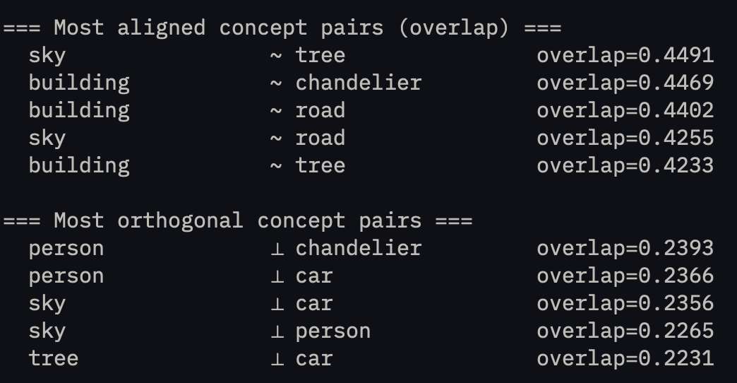Figure 13: Pairwise subspace overlap between semantic concepts

Conclusion

The DINOv3 model shows that for an image foundational model to be good at a range of downstream tasks it needs to both arrange features such that correlated object features are closer to each other, and it needs to identify semantic objects. So there seems to be a correlation with the fact that models need rich semantic features to be good at a wide range of computer vision tasks.